How to Create Drop Down List in Google Sheets with Color

If you’re wondering how to create a drop down list in Google Sheets with color, this is the guide for you! There are various times when you might want to create a drop down and then color code it based on the selection.

For example, maybe after finding duplicates in two columns, you'll want to categorize the data with a drop down list. Another use case for this might be if you are analyzing historical stock data and want to use repeated notes from a list. You could even add drop downs to your spreadsheet after syncing two sheets into one master sheet.

So, how do you create a color coded drop down list in Google Sheets? To create a drop down list in Google Sheets, you’re first going to use data validation to create the drop down. Next, you’ll want to set up conditional formatting to make the drop down selection color coded. The combination of using data validation and conditional formatting will give you the desired result!

Here are some step by step instructions for creating a dropdown list with color in Google Sheets.

Creating a Drop Down List Using Data Validation in Google Sheets

First, you’re going to click in the cell where you want the dropdown list to appear.

Next, click on Data in the top menu and then click on Data validation.

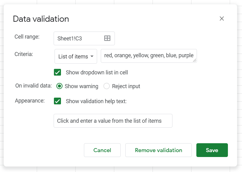
Next, you’re going to set the criteria for your drop-down list. You can create a drop-down list from only TWO of these criteria.

List from a range: This allows you to select a range of cells. Each cell will be a selection for the drop down.
List of items: Type a list of comma-separated items.

For this example, we will create a List of items for simplicity. To do this, select List of items and then type the list (comma separated) in the box next to the dropdown.

Additionally, make sure that the check box for Show dropdown list in cell is checked (it should be by default).

You can also choose to show a warning or reject the input on invalid data.

Lastly, you can choose to Show validation help text by checking the box and inputing what you want the text to display.

When finished, click Save.

After clicking Save, your cell will become a dropdown menu. You can copy this dropdown to any other cell that you would like the have the same menu options. Just like you can see here. I copied the cell in Row 2 (dropdown menus are indicated by a down arrow) and pasted another dropdown in row 3.

How to Use Conditional Formatting to Color Code Your Drop Down List

Here comes the fun part… conditional formatting!

To get started, you’re going to highlight the drop down cells that you want to color code. Then click on Format in the top menu and select Conditional formatting in the menu.

Next, a box will pop out on the right where you can start defining your color code.

In this example, because we have a text list, we’re going to select Text contains in the dropdown menu under Format cells if…

Then you’ll type in the text that you want to color code in the next text box.

Lastly, you’ll select the color in the Formatting style box and click Done.

Now you can see if green is selected from the dropdown menu, the entire box turns green based on the color selection chosen in the step above.

You can do the same thing for numbers that are greater than or less than. Additionally, you can set up multple conditions for the same range of cells if you wanted.

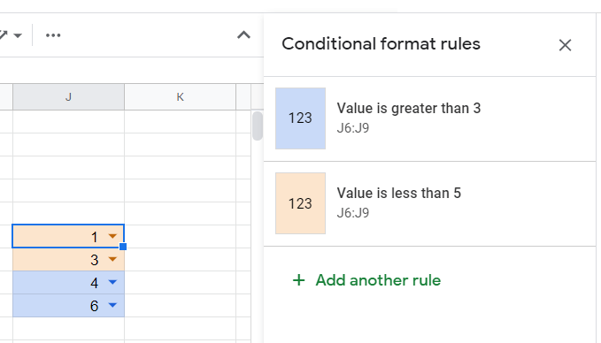
In this example, I’ve created drop down lists of numbers and set conditional formats for values that are greater than 3 but less than 5.

Keep in mind that if you have conditional formats that overlap like the one below, the rules at the top apply first.

For example, Value is greater than 3 means that only the 4 and 6 are highlighted blue.

However, Value is less than 5 should include the 1, 3, and 4 but since the the rule for Value is greater than 3 is first in the list of rules, those values are highlighted first.